In the previous article we assembled a first version of the metagenome, using a fast assembler creating a lot of rather small contigs. We need now to separate these reads according to the different genomes present in the assembly: this is called binning.
To tease apart the different genomes we are relying on several concepts:
- First the different bacterial OTU present in the genomes are certainly present in different abundance. Based on this we hope that the more one species is present in the sample, the more it’s genome will be represented in the total sequencing read (They should have a higher coverage). Note: The abundance (or coverage) of one bacterial species in the metagenome could also be affected by the DNA extraction method (this will probably be address in a further article)
- Bacteria from different group (Phylum/Class/even between Order) very often share different GC content and tetranucleotide usage frequencies.
Many tools have different approach to deal with this. In this post we are going to use a R package called Genome binning tool or gbtools, from another colleague of mine Brandon Seah. I will probably go over other tools in future posts. He’s approach is a simplified version of the work of Mad Albertsen on differential coverage genome approach (you can find the original paper here).
The gbtools package has been developed to give separate genomes from differential coverage technique when possible and by GC against coverage value. Using these values the contigs are then displayed on a graph which allow the user to visually identify different group of contigs or bins.
This package gives you a lot of freedom in selection of genomic bins by displaying contigs with tRNAs; essential or unique genes; or what ever you can think of. Brandon has a quite well explain wiki on his github page.
We are going to put our tongue metagenome through this package and see what we can take out of it.
Preparing the data
First we are going to run the assembly file through different software and scripts in order to get some general information from our assembly. We need to get the coverage values and GC content of all the contigs in the assembly. For this we use the mapper bbmap.sh from the BBmap suit.
bbmap.sh ref=final.contigs.fa in=reads_q2.fq.gz minid=0.98 covstats=coverage.stat
The covstats option is here very useful because it will generate a table almost ready to use with all the information we need. We use the option minid=0.98 which is going to only count the reads with a similarity around 98% to the reference (ref) (Note: bbmap has the tendency to select a minimum identity lower to what you input, you can see the exact value in the output).
Once we have the file “coverage.stat” it should look like this :
Section
#ID Avg_fold Length Ref_GC Covered_percent Covered_bases Plus_reads Minus_reads Read_GC

k99_5 40.8273 238 24.3109 238 0.4244 100.0000 238 32 26 0.4349

k99_7 8.0000 327 7.0336 327 0.4220 100.0000 327 11 12 0.4386

k99_8 6.0000 338 6.8047 338 0.2337 100.0000 338 12 11 0.2228

k99_9 3.0000 316 3.1646 316 0.2880 100.0000 316 4 6 0.2933

k99_10 2.0000 360 1.9444 360 0.3917 96.1111 346 4 3 0.3891

k99_11 67.9524 351 45.8405 351 0.3590 100.0000 351 78 83 0.3407

k99_12 189.2240 291 158.9691 291 0.4433 100.0000 291 236 227 0.4469

k99_13 8.6139 415 8.9157 415 0.3542 97.3494 404 17 20 0.3240

k99_14 24.3911 301 19.6013 301 0.3189 97.6744 294 25 34 0.3172

k99_15 12.0000 375 5.8667 375 0.3920 98.4000 369 10 12 0.3848
The first # symbol of the file needs to be removed to be processed correctly by the gbtool package later.
We are going to look for ribosomal sub units makers, for this we use one of the accessory scripts of the gbtools package:
perl get_ssu_for_genome_bin_tools.pl -d <path/to/ssu/database> -c -a final.contigs.fa -o assembly.ssu
This script rely on a V-indexed database identical to the one used by phyloFlash. If you previously used it, you can use the same database. The path to the database should look like /PATH/TO/phyloFlash/119/SILVA_SSU.noLSU.masked.trimmed.fasta. (119 is the silva version)
Then we are going to detect tRNA and uniques genes in order to assess the completeness of the different bins present in the assembly. For this we run :
tRNAscan-SE -G -o tRNA.tab final.contigs.fa
tRNAscan as the name suggests it is a fast software to detect all the tRNA sequences present in the assembly.
perl /tool/AMPHORA2/Scripts/MarkerScanner.pl -DNA -Bacteria final.contigs.fa

perl /tool/AMPHORA2/Scripts/MarkerAlignTrim.pl --WithReference --Output phylip

perl /tool/AMPHORA2/Scripts/Phylotyping.pl > amphora.results

mkdir Amphora

mv *pep Amphora

mv *mask Amphora

mv *phylotype Amphora

mv *aln Amphora

perl /tool/genome-bin-tools/accessory_scripts/parse_phylotype_result.pl -p phyla.results > phyla.results.parsed

perl /tool/genome-bin-tools/accessory_scripts/parse_phylotype_result.pl -p amphora.results > amphora.results.parsed
Amphora2 and Phyla Amphora a two software devellopped by Martin Wu, they both detect essential/unique genes from different organisms in the different contigs. They both operate on a different taxonomic level: Amphora2 is going to detect different gene set from different Kingdom to the class level, whereas PhylaAmphora will predict genes on the order/family level.
The script above has a some commands to order the different file generated by both Amphora and Phyla Amphora scripts. But once generated you could very well delete these intermediate files. The two last commands are from the gbtools package to format the *Amphora output to be processed in R smoothly.
>k99_5 flag=0 multi=40.8273 len=238
There are space in the name, and some script like bbmap can deal with them and other don’t like Amphora2 and PhylaAmphora. So there is two solution here:
- You change the name in the initial assembly file, by replacing all space by an underscore for example. With for example the following command:
sed 's/ /_/g' final.contig.fa > final.good.name.fa
- You do some command juggling and you try something overly complicated and not very elegant if you don’t want to wait again for the previous script to run again. You need to modify the table file to have the sequence names be the same name as in the Amphora file. The amphora file didn’t keep anything in the name after the first space. We do something like this :
cat table.file | awk '{FS=" "}{print $1}' > temp

cat table.file | awk '{FS="\t"}{ for(i=2; i<NF; i++) printf "%s",$i OFS; if(NF) printf "%s",$NF; printf ORS}' > temp2

paste temp temp2 > temp3

sed 's/ /\t/g' temp3 | sed 's/\t\t/\t/g' > table.adjusted.file

rm temp*
The first line print the first column if you consider the file to have space as a field separator, and stores it in a temporary file, this allows us to keep the same name as well as the header . The second line actually print all column except the first one if you consider the file to have tab field separator and stores is in another temporary folder. Then we paste post temp folder together, but then I realize a little snafu with the separator being space and not tab. Oh well let’s just replace them into a new fresh table file and remove the other temp.
If you have a simpler way to do this, I am happily taking suggestions.
Finally, we Plot !
Now we have everything. We can then start to use Gbtools with R. To load the data we are going to use the following command:
library("gbtools")

d<-gbt(covstat=, mark=amphora.results.parsed, marksource="PA", trna="tRNA.tab", ssu="assembly.ssu.tab")
Now we can finally plot all our information. We are going to plot the contig according to their coverage value and GC content, then we are going to overlay unique gene colored by taxonomy.
plot(d, legend=TRUE, ssu=TRUE,textlabel=TRUE)
Legend add the taxonomy color legend of the Amphora markers, ssu and text label label contigs with identified Ribosomal subunit and their name.
It should now look like this:
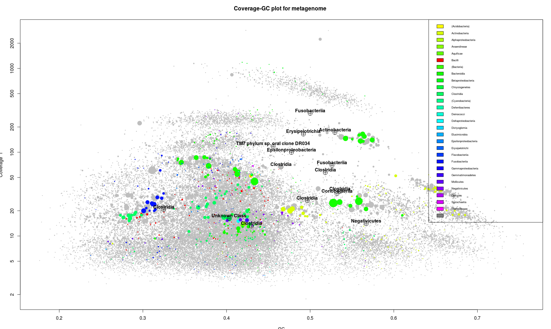
This picture contains a lot of information. The position and the clustering of the dots, indicates groups of sequences which are likely to belong together. Following this, each elongated little cloud would be a single bacterial genome. On the graph we can identify around 8 different groups of contigs. Likely to be 8 different genomes.
Also each one of these little cloud is associated to one color, which is a good thing indicating that they regroup unique genes from the same bacterial class. We can see the color distribution across the plot and have a better idea of what’s actually dominating the sample. In our case probably bacterioidetes and/or betaproteobacteria (the green color).
Let’s focus first on what we can easily identify, isolate and and analyze.
The best feature of the gbtools package is the ability to select a part of the plot and have a look of what is in it.
We didn’t closed the previous window plot because it will be used with the the following command to place dot on the graph to circle our region of interest:
bin1 <- choosebin(d, slice=1)
Note
In the center we have a huge blob which correspond to all the bacterial sequences which are present in the same abundance and share a common GC value. This article will try to go through this mix of sequences, but it illustrate the limit of this approach. If some organisms are not sticking out by abundance or GC value it become difficult to separate them. Fortunately there are some way around this, mainly based on the use of a different binning method.
- Paired end mapping of the reads we could tract which contigs are linked together.
- Adding tetranucleotide frequency to the analysis, tools like metawatt performs these kind of analyses.
- Differential coverage. This method rely on the sequencing of the same sample by different DNA extraction methods or the sequencing of two related samples where some of the partner would have different abundance (coverage).
It is likely that each of these methods will have a dedicated article later on this blog
Note: slice=1 mean that the point are to be displayed on the coverage against gc of the first table. This option is important if we have another coverage information table (Will be discussed in another article). By default choosebin use 6 dots, if you want more than 6 points use the following
bin1 <- choosebin(d, slice=1, num.points=10)
Now we click on the picture and place 6 dot around on of the cluster of contigs we are interested in, as illustrated below.
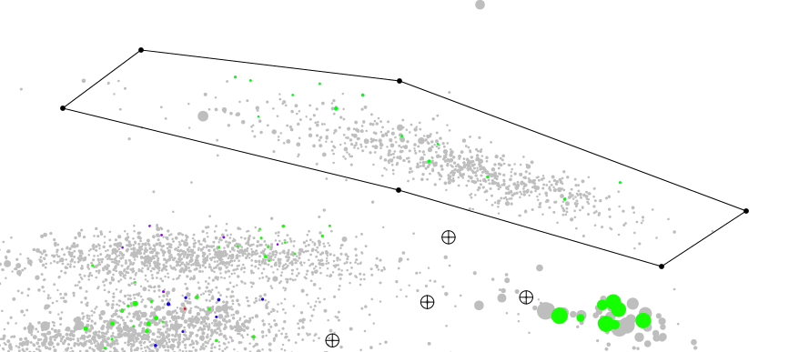
Note
Here I would like to mention, I deliberately did not include any SSU sequence in the bin while plotting. 16S rRNA sequences are conserved accross the bacterial kingdom, and as you can see on the first plot above, they tend to gravitate in the same area, because they have more or less the same GC content; and depending of how many copies there is in the genome their coverage value is skewed. It is common for these sequences to be located outside their respective cluster of contigs
In some case it is easy to correlate a SSU sequence to a specific bin. Here it seems that there is only one Fusobacteria bin and one Fusobacteria SSU sequence. In other case it is more complicated like here for the clostridia and the actinobacter where there is multiple bin and multiple SSU sequences.
In some case the paired end connectivity can resolve this problem, it will be discussed elsewhere.
Ok now what ? you got me through this all process for what ? A fancy way to make boxes ?
Yes! More or less ! But informative fancy boxes !
If we just type this in the R console:
bin1
We will have the following information:
> bin1

*** Object of class gbtbin ***

*** Scaffolds ***

Total Scaffolds Max Min Median N50

1 2276742 1710 49675 200 869.5 1280

*** Markers ***

Source Total Unique Singlecopy

1 A2 43 31 21

*** SSU markers ***

[1] 1

*** tRNA_markers ***

[1] 59

*** User-supplied variables ***

[1] ""

*** Function call history ***

[[1]]

gbt.default(covstats = "coverage.good.csv", mark = "amphora.results.parsed",

marksource = "A2", ssu = "tongue.ssu.ssu.tab", trna = "tRNA.tab")

[[2]]

choosebin.gbt(x = d, slice = 1)
This report tells us that the bin we selected regroups 43 known marker from Amphora2. This software uses 31 marker genes, here we have all of them present in the bin and 10 are present multiple time. From now we cannot tell if it is a real information, duplication of some of these genes, it can happen or if we have a mix of genomes/strains.
However it is likely that we have isolated most of a bacterial genome. In the next articles we are going to see how we can now improve this genome. But we are not done here yet.
If you type the following:
write(as.character(bin1$scaff$ID),file="shortlist.file")
And you will save in the file shortlist.file all the contig name isolated in bin1. It will be used with a small script to extract the related fasta reads from the initial assembly file. Here we use faSomeRecords from Jim Kent github.
faSomeRecords final.contigs.fasta shortlist.file bin1.fasta
here the first file is the initial assembly, the second one the shortlist and the last one the name of the new file with the extracted sequences.
We can now repeat the process and select/extract all these clusters of contigs easy to spot.
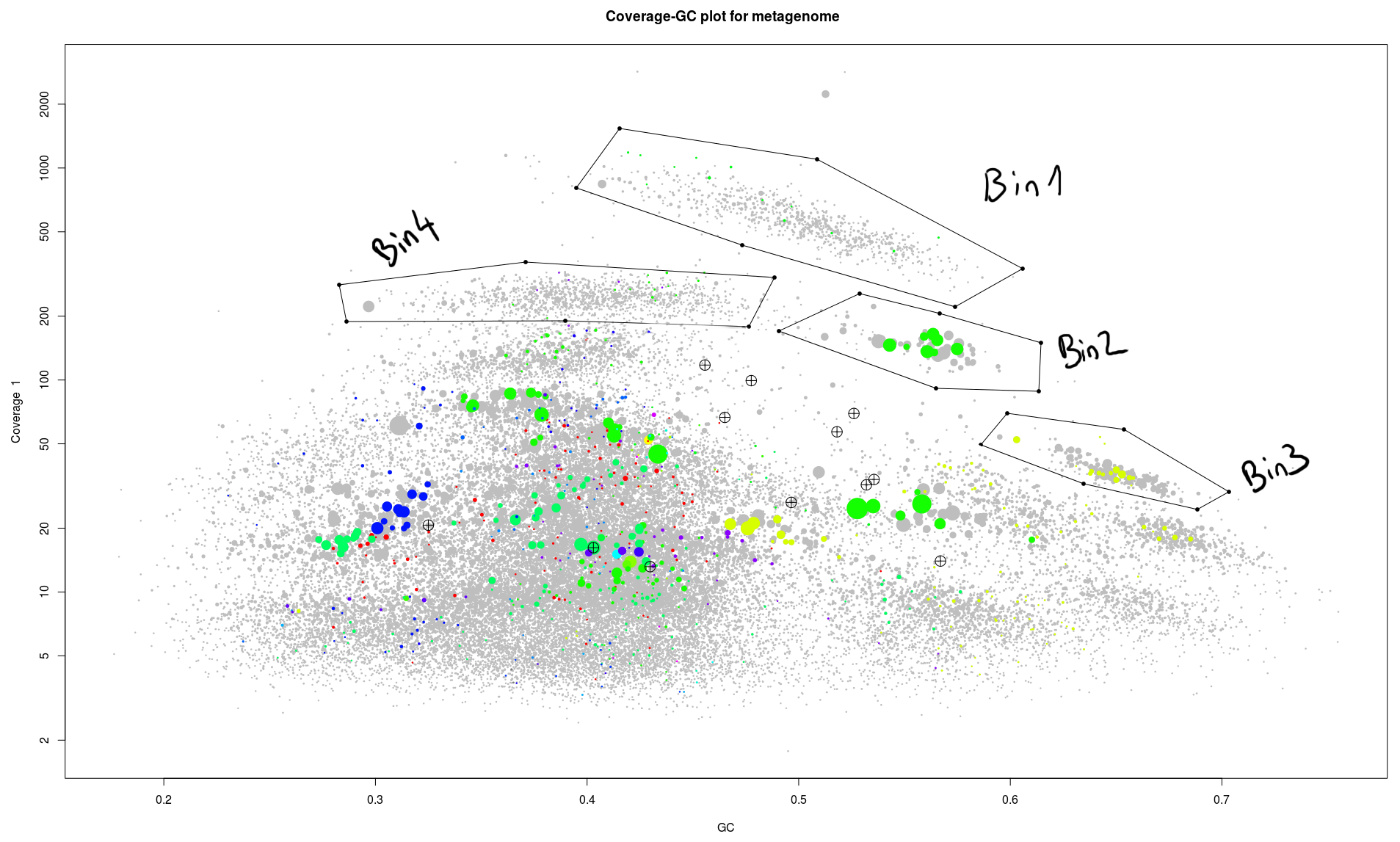
So we have four bins which are apparently easy to circle out of the rest of the genome.
Below are the stat of each one.
> bin2

*** Object of class gbtbin ***

*** Scaffolds ***

Total Scaffolds Max Min Median N50

1 2276427 146 145256 202 1109 342

*** Markers ***

Source Total Unique Singlecopy

1 A2 32 31 30

*** SSU markers ***

[1] 1

*** tRNA_markers ***

[1] 62

*** User-supplied variables ***

[1] ""

*** Function call history ***

[[1]]

gbt.default(covstats = "coverage.good.csv", mark = "amphora.results.parsed",

marksource = "A2", ssu = "tongue.ssu.ssu.tab", trna = "tRNA.tab")

[[2]]

choosebin.gbt(x = d, slice = 1)
> bin3

*** Object of class gbtbin ***

*** Scaffolds ***

Total Scaffolds Max Min Median N50

1 2255929 261 97625 211 4402 10738

*** Markers ***

Source Total Unique Singlecopy

1 A2 39 27 20

*** SSU markers ***

[1] 0

*** tRNA_markers ***

[1] 47

*** User-supplied variables ***

[1] ""

*** Function call history ***

[[1]]

gbt.default(covstats = "coverage.good.csv", mark = "amphora.results.parsed",

marksource = "A2", ssu = "tongue.ssu.ssu.tab", trna = "tRNA.tab")

[[2]]

choosebin.gbt(x = d, slice = 1)
> bin4

*** Object of class gbtbin ***

*** Scaffolds ***

Total Scaffolds Max Min Median N50

1 4036419 1231 128931 205 1945 1738

*** Markers ***

Source Total Unique Singlecopy

1 A2 66 31 10

*** SSU markers ***

[1] 0

*** tRNA_markers ***

[1] 74

*** User-supplied variables ***

[1] ""

*** Function call history ***

[[1]]

gbt.default(covstats = "coverage.good.csv", mark = "amphora.results.parsed",

marksource = "A2", ssu = "tongue.ssu.ssu.tab", trna = "tRNA.tab")

[[2]]

choosebin.gbt(x = d, slice = 1)
- We can see that bin 2 seems to be very nice, 2mb total, only one duplication of the marker genes a lot of tRNAs (maybe too much).
- Bin3 is around 2,2mb which is normal for bacteria and has a lot of marker genes, but only 27 unique ones, four are missing. Maybe we just missed them while drawing the contours. We might catch them in one of the later steps.
- For Bin4 it start to be less obvious, we have a genome size of 4mb, 66 maker genes, where 21 are present multiple time. Here we might have two genomes overlapping in this selection. We are going to have a look at this case in the next blog post.
We started to isolate genomic bins, but we still have a lot to do with the current assembly file. We are going to end here for this blog post. In the next article we will try to handle the extraction of the less evident bins. Then we will see what to do with these bins.