We continue the analysis of a metagenome library coming from a sample of the dorsal tongue of SRS147120. After the previous article we now we know what to expect in the metagenomic library. We have quite a diversity of predicted OTU.
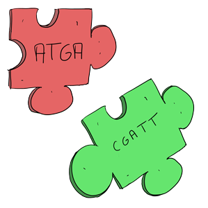
It is time to do the first round of assembly. First to explain the challenge we face, one analogy I like (probably coming from somewhere on SEQanswer) is to consider a metagenome reads like a puzzle piece. And right now you are facing a mountain of puzzles pieces. You don’t know if the pieces are coming from different sets and worse you don’t know if you have all the pieces. If you try assemble the different puzzles piece by piece this it might take forever. Fortunately we have way to speed up the process.
We want to have a first quick and unspecific assembly. From our previous analyses we know that we might expect 5 to 10 at least partial bacterial genomes in the library and probably more are present but probably largely incomplete.
We are going to use this two concept to separate the mountain of puzzle pieces to smaller piles easier to handle but we will come back to this after the assembly. In a first time we want to use as much read as possible to build as much contigs (sequence composed of an assembly of reads) from the whole metagenome.
The assembling software should not spend too much time and resources trying to figure things out. Software like IDBA-UD or the latest version of Megahit, are very good a this. From a huge library (like our example here with 100 millions reads) these software will generate a lot of small contigs.
For this example we use megahit and run the following command:
megahit --12 reads_q2.fq.gz -o assembly
Quite simple command. The defaults options of the latest version of megahit allow to automatically scale the parameter to the system performances. –12 means we have a interleaved assembly (which is compressed) and -o is the output folder.
When the assembly is done, we can use a script to have a summary of what it look like. Here we use Quast, which tell us how many contigs we have, what is the longest one, and what is the N50 of the length of the different contigs.
The command is :
quast.py -o MG_quast final.contigs.fa
Which is going to output us different report format in the -o folder. The report.txt is as follow:
All statistics are based on contigs of size >= 500 bp, unless otherwise noted (e.g., "# contigs (>= 0 bp)" and "Total length (>= 0 bp)" include all contigs).

Assembly final.contigs

# contigs (>= 0 bp) 182720

# contigs (>= 1000 bp) 38099

Total length (>= 0 bp) 184324935

Total length (>= 1000 bp) 111708906

# contigs 97387

Total length 152576288

Largest contig 342016

GC (%) 41.63

N50 2094

N75 952

L50 12591

L75 40892

# N's per 100 kbp 0.00
If we look at the contig with more than 1000 bp we can see above that this assembly round regroups 38000 contigs for more around 111Mb of total prokaryotic (proably) DNA.
The latest version of Megahit allow us to have a look at the de brujin connectivity between the different contigs. At one stage of the assembly, the algorithm tries to check which contig is likely to connect with another, partially with the paired end information. But often it breaks, because the support is not enough, or multiple possibility exist (in the case of polymorphism or repeat region such as mobile element for example.) And this information can be summarized in a fastg format.
The wiki from megahit advise to use one of the assembly iteration to generate the Fastg file because some of the uncertain contigs could have be filtered in the last step. The command:
megahit_toolkit contig2fastg 99 ./intermediate_contigs/k99.contigs.fa > k99.fastg
The first number is the kmer size you want to use to generate the graph, and then you call the corresponding iteration contig file to finaly pipe the result in you fastg output.
This file can then be visualized with specific software like Bandage. This software, a bit complex to install sometime, generate a graphical representation of the contig network. And has a very useful blast search function incorporated. When we load our fastg file and ask to draw the whole network based on the initial assembly we have a huge picture of the thousands of contigs represented. Because looking at the overall representation of the network is not going to fit in this post (but you can see it here, -warning- it is a large picture), we are going to have a closer look a different examples :
Each colored line represent a single contig. Black lines are connecting the different contigs based on the de Brujin graphs.
On the top of the representation we have a few big complex bundle of lines. These networks probably represents some of the most completes bacterial genomes present in the assembly. These huge network are good starting point to tease apart the different player in the genomes. But very similar region in bacteria like the 16S rRNA sequences could be miss placed in such bundle.
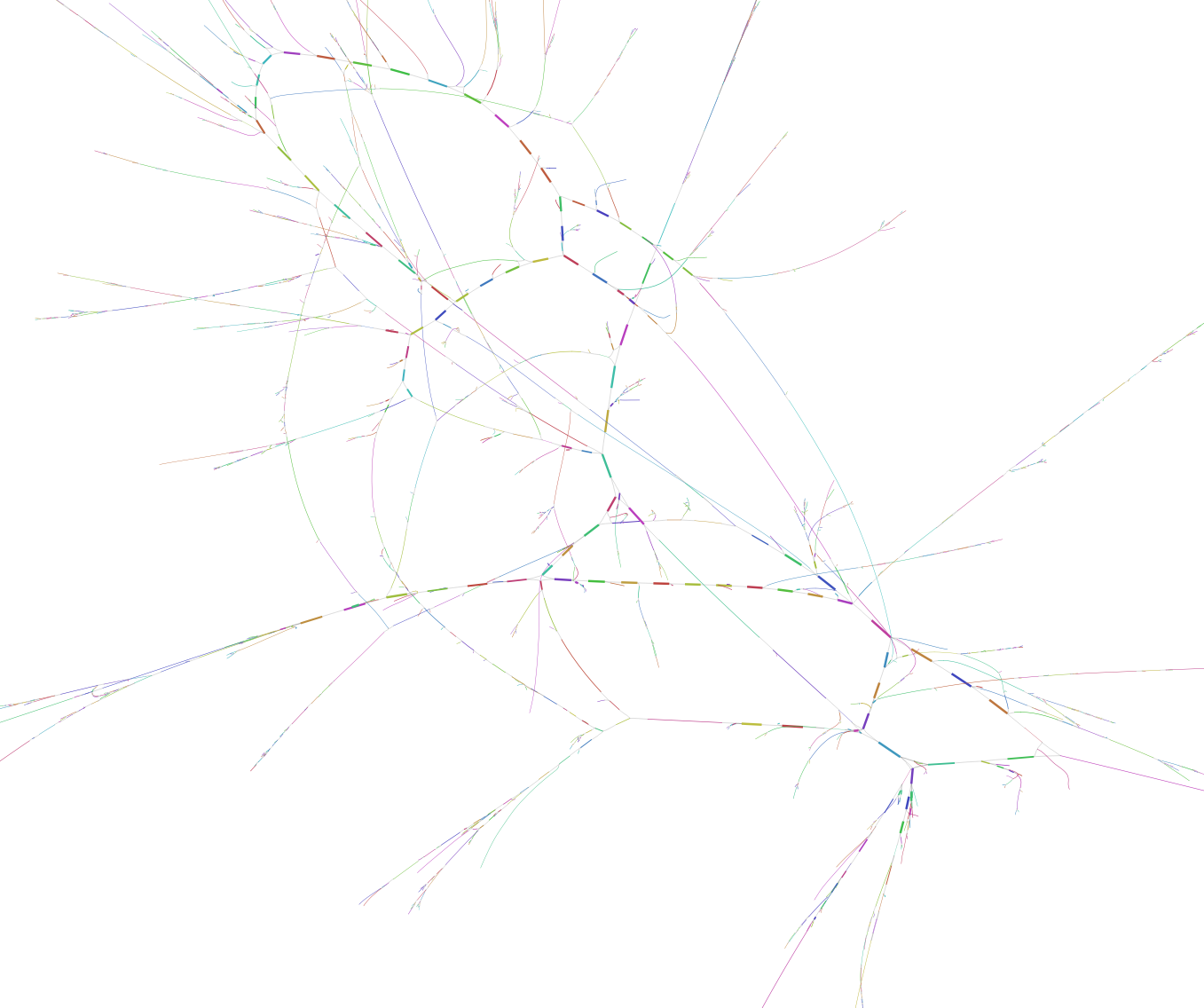
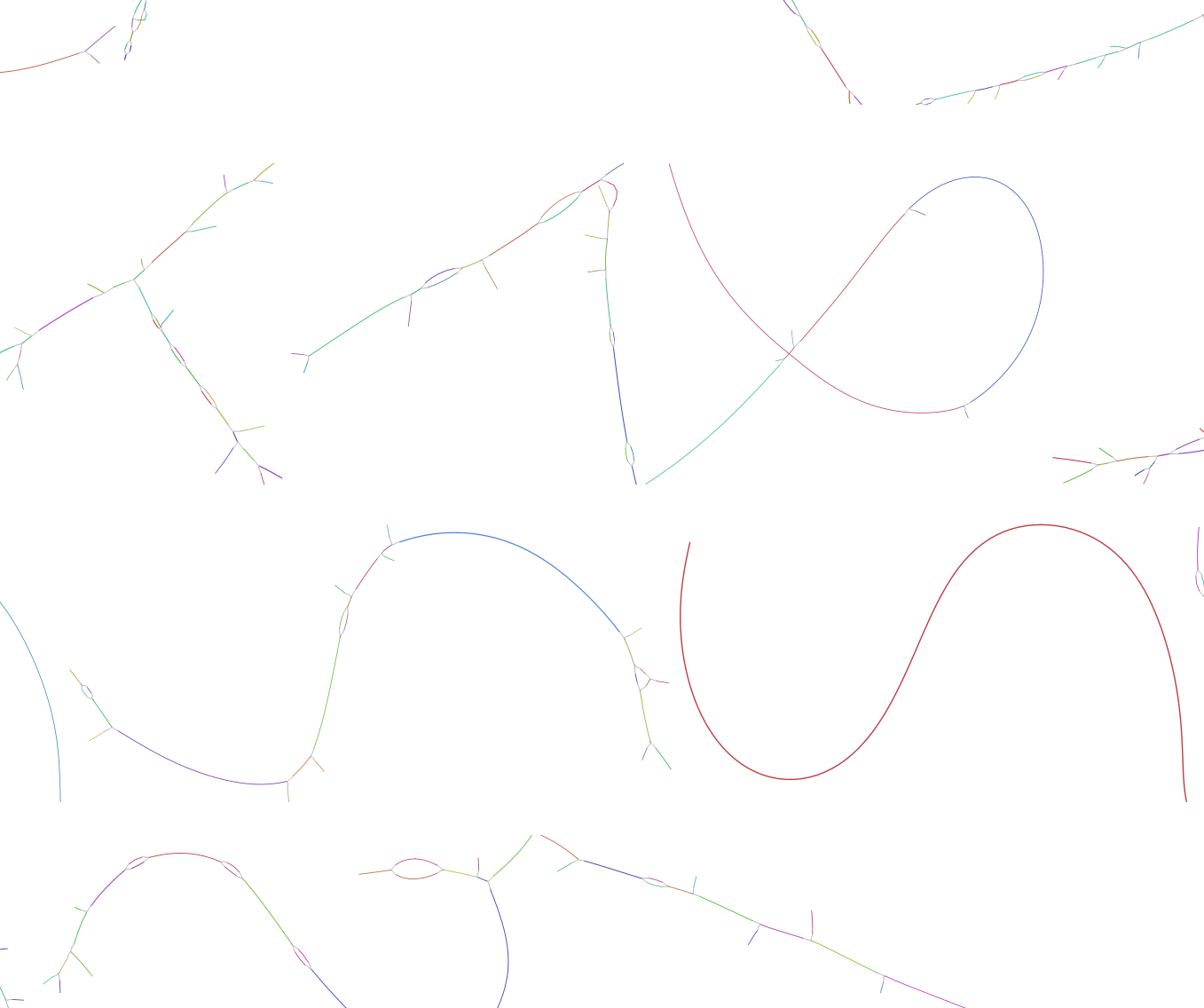
On the lower part of the representation are displayed single contigs and smaller networks. These fragments have not been placed in connection with anything else. There is multiple explanation for this:
- The contig/small network is from a bacterial genome present in only very low abundance and nothing else connects to it.
- This contig is a repeat element and connect to too many other network/contig and can not be reliably assigned to one specific network.
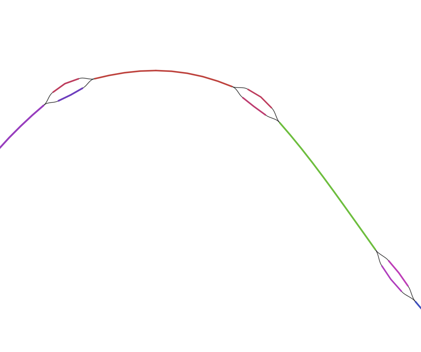
On the left is a representation of the assembler not knowing which contigs goes where. A single large contig is connected to two small ones, the smaller contigs are probably repeated elements such as transposases, which are very identical and can’t be assigned reliably to a larger set.
With bandage we can select and export the different big networks and save them as single fasta file. We are going to use them later in our binning process.
In the next post we are going to dive in depth in a efficient method to separate the different genomes in our big messy assembly.