![[Playing with Data] Looking at a Fish pathogen genome](http://www.aassie.net/Pro/wp-content/uploads/2016/08/Cropped.Banner.png)
In this blog note I will use some of the techniques I used in my previous post to look at a recently published dataset.
Last year I came across a study by the Institute for Veterinary Pathology, in Zürich, Switzerland describing a bacterial pathogen of fish. Aquaculture is a big business and can invest into understanding what kind of pathogens infect their stocks. This study looked at sharpsnout seabream (Diplodus puntazzo) larvae reared in mesocosm cultures. This is a technique where the fish basins are connected to an unfiltered sea water source to mimic natural environment and provide the fish with plankton to feed on. They selected and analyzed individual larvae which were developing infectious cysts.
The study describes the bacteria thriving in those cysts. With genomic analysis they showed that the pathogen is certainly a new species in the Endozoicomonas genus and they confirmed that these guys were the main infectious bacteria using Fluorescence in situ Hybridisation (FISH). In our lab we are interested in a sister genus (*spoilers*) and I was curious to see what lies in the genome of these bacteria. I decided to start the analysis from the original reads and assemble the pathogen genome the same way as the one we have in house to compare them using the same techniques.
And so after playing with reads for a few days I wanted to share the results.
The study is based on three different datasets all sequenced with the Illumina sequencing platform.
- The first one is composed of DNA coming from a micromanipulated cyst, and where part of the DNA was amplified with MDA (multiple displacement amplification) and pooled back with the original DNA, then sequenced.
- The second comes from the DNA of an entire larvae (21 day after hatching) the host DNA was then depleted and the remaining DNA amplified with MDA.
- And the last one is the sequencing of DNA extracted from an infected larvae tail.
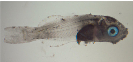
A sharpsnout seabream larvae heavily infected with epitheliocystis affecting fins and skin. Isn’t it beautiful ?
After downloading the data from the ENA server we post-processed the illumina reads with one of the scripts from the bbmap suite. We used the following parameters on the three separate libraries independently.
bbduk.sh in=RAW_Lib1_R1.fq.gz in2=RAW_Lib1_R2.fq.gz qtrim=rl trimq=25 ref=bbmap/ressource/nextera.fq.gz,bbmap/ressource/trueseq.fq.gz,bbmap/ressource/phix174_ill.ref.fa.gz out=Lib1_R1.fq.gz out2=Lib1_R2.fq.gz
This operation is going to remove contaminants and bad quality reads. qtrim=rl will trim on both ends of the reads, trimq=25 will remove any base with a quality below 25, ref=… removes contaminant sequences from the library preparation (I put here both nextera and trueseq reference files because depending on the protocol one of the two primer sets could have been used).
The first assembly
Then we assembled the three libraries individually, using megahit.
megahit -1 Lib1_R1.fq.gz -2 Lib1_R2.fq.gz -o Lib1_Megahit
This outputed a new folder called Lib1_Megahit containing the assembly file. To find out what is in our library, we used a protocol described on the gbtool github page. This protocol will enable a visual representation of the different assembled contigs and their phylogenetic affiliation.
We next checked for the presence of tRNA in this assembly, which will help us later to evaluate the quality of the assemblies and bin selection. For this we used:
tRNAscan-SE -G -o Lib1.trna.tab Lib1_Megahit/final.contigs.fa
To use the gbtools script, we needed to first generate accessory files to get contigs coverage and taxonomic information. To do this we mapped the assembly reads using bbmap as follows:
bbmap.sh ref=Lib1_Megahit/final.contigs.fa in=Lib1_R1.fq.gz in2=Lib1_R2.fq.gz minid=0.98 covstats=Lib1_mapped_Lib1.tab

bbmap.sh ref=Lib1_Megahit/final.contigs.fa in=Lib2_R1.fq.gz in2=Lib2_R2.fq.gz minid=0.98 covstats=Lib2_mapped_Lib1.tab
With this information multiple thing can be done to visualize the data. First, if we had only one metagenomic library, we would have plotted the coverage value of each contigs against their average GC content. Sometime the difference of average content between host and bacteria is enough to identify a bacterial bin.
However, here we could use the other libraries used in the publication and used differential coverage to bin the different genomes in the early metagenomic assembly. We have very similar metagenomic libraries, two coming from the same fish larvae and the other from the same batch of individual. Because we can expect that the host and pathogens are relatively the same, we bet that the short reads from one libraries is going to map to another one, being not sensitive enough to pass small strain/individual genetic variation. But we also bet that the pathogen is present in different abundance in the different samples, making the differential coverage a method to disentangle the bacterial bin.
Megahit include spaces in the names of the output contigs. The different scripts used below do not like this and will keep as the contig name only the first “word”. A little scripting exercise is needed to adjust the names in the coverage files.
 cut -d " " -f 1 Lib1_mapped_Lib1.tab | cut -f 1 > temp

cut -f 2-9 Lib1_mapped_Lib1.tab > temp2

paste temp temp2 > Lib1_mapped_Lib1.tab

rm temp*
Then we used one of the gbtools accessory scripts to have an idea of the taxonomic affiliation of some of the contigs. This script is based on the blobology software.
perl tools/genome-bin-tools/accessory_scripts/blob_annotate_mod.pl --assembly E1.Megahit/final.contigs.fa --blastdb /Path/to/ncbi/nt --out Lib1.contig_taxonomy.tab --num_threads 30 --taxdump /Path/to/ncbi_taxdump/
Now we can now run the gbtools script in R.
R

> library('gbtools')

> Lib1<-gbt(covstat=c("Lib1_mapped_Lib1.tab","Lib2_mapped_Lib1.tab"), marksource="Blob", mark="Lib1.contig_taxonomy.tab", trna="Lib1.trna.tab")

> plot(Lib1, slice=c(1,2), legend=T)
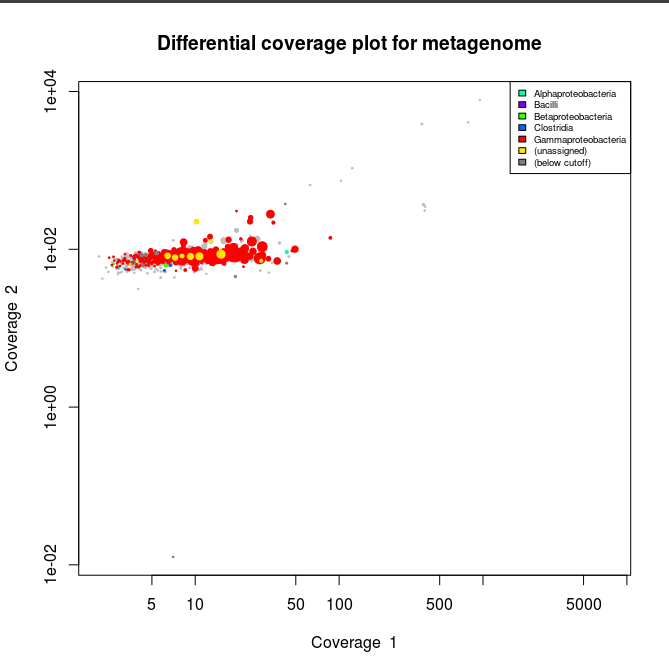
This applied to the three libraries will output the following schematics, where each dot represent an assembled contig displayed with its coverage values and colored according to its taxonomical affiliation.
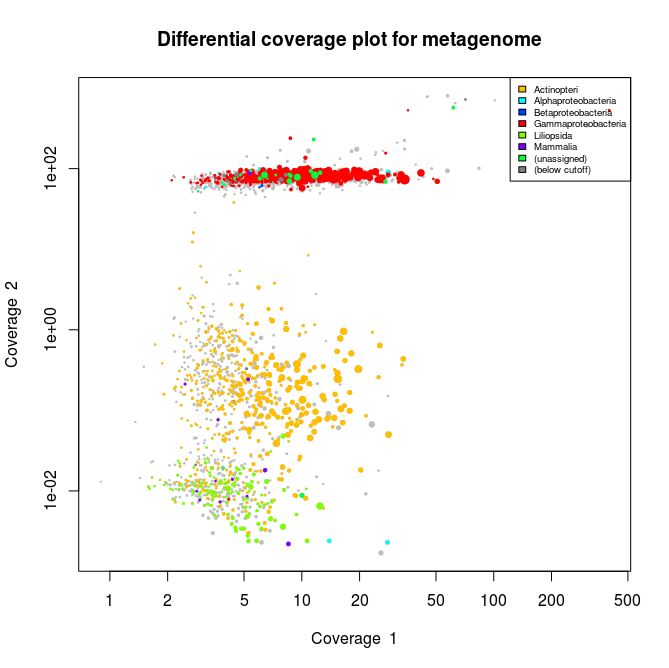
Library 1 plot. In red are the contigs related to Gammaproteobacteria
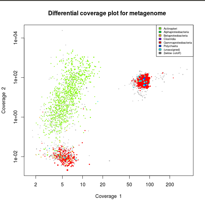
Library 2 plot. In red are the contigs related to Gammaproteobacteria. Note here that there appear to be two different bins related to the Gammaproteobacteria
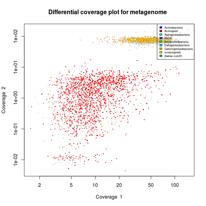
Library 3 plot. In orange are the contigs related to Gammaproteobacteria
What we can see from the plots above, is the clear presence of two main organisms in the metagenomes. In all libraries we see a cluster of contigs related to the Gammaproteoabcteria and the Actinopteri.
The Actinopteri is a group of fish so these huge clouds are the host. In the first and the third library the gammaproteobacterial clouds are likely to be the Enodozoicomonas related reads.
Then in the first and the second libraries we can see a third cluster of reads. In the first library they are related to either unassigned taxonomy or Liliopsida group. Which is a group of plants… It is unlikely to be real, probably a contamination from the sequencer if the samples were sequence before/after/at the same time as other unrelated samples. In the case of the second library, the most covered bin is likely to be the Endozoicomonas bin, but I also assemble a second bin present with a lower coverage. This bin might be discussed in another post.
Now we wanted to get the gammaproteobacterial related bins! To do so:
>Lib1_bin1 <- choosebin(Lib1, slice=c(1,2))
This allows us to interactively choose the part we want to extract like shown on the picture below.
We can inspect this bin by just typing Lib1_bin1 and this will output a summary of how many marker genes and how much tRNA is present in the selected bin.

When you type Lib1_bin1 you will get :
*** Object of class gbtbin ***

*** Scaffolds ***

Total Scaffolds Max Min Median N50

1 5528397 2050 42385 201 1225.5 5828

*** Markers ***

Source Total Unique Singlecopy

1 blob 610 0 0

*** SSU markers ***

[1] NA

*** tRNA_markers ***

[1] 74

*** User-supplied variables ***

[1] ""

*** Function call history ***

[[1]]

gbt.default(covstats = c("Lib1_mapped_Lib1.tab", "Lib2_mapped_Lib1.tab"),

mark = "Lib1.contig_taxonomy.tab", marksource = "blob", trna = "Lib1.trna.tab")

[[2]]

choosebin.gbt(x = d, slice = c(1, 2))
If we are satisfied with the bin evaluation, I can proceed with extracting the contig names by doing:
> write.gbtbin(Lib1_bin1,file="Lib1_Bin1.shortlist")
This can then be used to extract the original contigs from the assembly file using faSomeRecords (from the kentUtils package)
faSomeRecords E1.Megahit/final.contigs.fa Lib1_Bin1.shortlist Lib1_Bin1.fasta
Now we have all the reads related to the gammaproteobacterial bin. We can then start to reassemble the reads to try to improve the bin in a proper draft genome.
The reassembly
So for the specific gammaproteobacterial reassembly we first gathered the reads mapping to the bin we just extracted from the initial assembly. To do so, we used bbmap as follow:
bbmap.sh ref=Lib1_Bin1.fasta in=Lib1_R1.fq.gz in2=Lib1_R2.fq.gz minid=0.98 out=IT1/Lib1_IT1.bin1.fq.gz outputunmapped=f
We want the reads mapping the closest to our contig bin, so I set up minid=0.98 to have only reads mapping with 98% to the reference. We set set the output reads in an interleaved format for logistic purpose, too many files in a folder get confusing.
We can then assemble the reads with a more sensitive assembler such as SPAdes. In this case we use the single cell mode of SPAdes (–sc).
spades.py --sc --pe1-12 Lib1_.IT1.bin1.fq.gz -o Lib1_bin1.it1.spades
So from here we go once again with the gbtool protocol as follow:
#Mapping

bbmap.sh ref=Lib1_bin1.it1.spades/scaffolds.fasta in=Lib1_R1.fq.gz in2=Lib1_R2.fq.gz minid=0.98 covstats=Lib1_bin1.it1.mapped_Lib1.tab

bbmap.sh ref=Lib1_bin1.it1.spades/scaffolds.fasta in=Lib2_R1.fq.gz in2=Lib2_R2.fq.gz minid=0.98 covstats=Lib2_bin1.it1.mapped_Lib1.tab
#Taxonomy scan

perl tools/genome-bin-tools/accessory_scripts/blob_annotate_mod.pl --assembly Lib1_bin1.it1.spades/scaffolds.fasta --blastdb /Path/to/ncbi/nt --out Lib1_bin1.it1_taxonomy.tab --num_threads 30 --taxdump /Path/to/ncbi_taxdump/
#Gbtool

R

> library('gbtools')

> Lib1<-gbt(covstat=c("Lib1_bin1.it1.mapped_Lib1.tab","Lib2_bin1.it1.mapped_Lib1.tab"), marksource="Blob", mark="Lib1_bin1.it1_taxonomy.tab") > plot(Lib1, slice=c(1,2), legend=T)

> plot(Lib1, slice=c(1,2), legend=T)
Now the plots appear to have mainly gammaproteobacterial contigs. And when we check the stats :
>Lib1

*** Object of class gbt ***

*** Scaffolds ***

Total Scaffolds Max Min Median N50

1 5461446 1463 50576 78 1346 10265

*** Marker counts by source ***

Blob

536

*** SSU markers ***

[1] NA

*** tRNA markers ***

[1] 57

*** User-supplied variables ***

[1] ""

*** Function call history ***

[[1]]

gbt.default(covstats = c("Lib1_bin1.it1.mapped_Lib1.tab", "Lib2_bin1.it1.mapped_Lib1.tab"),

mark = "Lib1_bin1.it1_taxonomy.tab", marksource = "Blob")
We can see that after isolating our gammaproteobacterial bin we double the N50 size of the contigs. Now we can check for bin completion/contamination and heterogeneity using the checkm software.
Two folders checkm_bin and checkm_out are created and we placed the different gammaproteobacterial bins in checkm_bin and run the following command:
checkm lineage_wf -x fasta checkm_bin checkm_out
And we get this summary :
| Bin Id | Marker lineage | # genomes | # markers | # marker sets | 0 | 1 | 2 | 3 | 4 | 5+ | Completeness | Contamination | Strain heterogeneity |
|---|---|---|---|---|---|---|---|---|---|---|---|---|---|
| Lib1.it1.scaff | c__Gammaproteobacteria (UID4444) | 263 | 507 | 232 | 42 | 452 | 12 | 0 | 1 | 0 | 89.55 | 3.71 | 0.00 |
| Lib2.it1.scaff | c__Gammaproteobacteria (UID4444) | 263 | 507 | 232 | 4 | 492 | 7 | 3 | 0 | 1 | 98.98 | 5.32 | 3.23 |
| Lib3.it1.scaff | c__Gammaproteobacteria (UID4444) | 263 | 507 | 232 | 20 | 471 | 13 | 2 | 0 | 1 | 94.04 | 6.20 | 14.71 |
Along with this statistics:
Lib1.it1.scaff
Translation table: 11
GC std: 0.03796278225660953
# ambiguous bases: 931
Genome size: 5461446
Longest contig: 50576
N50 (scaffolds): 10265
Mean scaffold length: 3733.045
# contigs: 1536
# scaffolds: 1463
# predicted genes: 6026
Longest scaffold: 50576
GC: 0.4661748937600208
N50 (contigs): 9557
Coding density: 0.8327466755141404
Mean contig length: 3555.0227864583335
Lib2.it1.scaff
Translation table: 11
GC std: 0.038327815407111054
# ambiguous bases: 0
Genome size: 6200340
Longest contig: 91405
N50 (scaffolds): 20792
Mean scaffold length: 9025.24
# contigs: 687
# scaffolds: 687
# predicted genes: 6252
Longest scaffold: 91405
GC: 0.4680682027114642
N50 (contigs): 20792
Coding density: 0.8343495679269202
Mean contig length: 9025.24017467249
Lib3.it1.scaff
Translation table: 11
GC std: 0.037723956009137534
# ambiguous bases: 58
Genome size: 5518539
Longest contig: 41171
N50 (scaffolds): 5657
Mean scaffold length: 3164.29
# contigs: 1745
# scaffolds: 1744
# predicted genes: 6318
Longest scaffold: 41171
GC: 0.4719407387648884
N50 (contigs): 5657
Coding density: 0.8308628425023362
Mean contig length: 3162.4532951289398
So from the list above we can see that the individual assembly yielded bins with quite high completeness scores. On the statistic part the draft genome from the three libraries also share globally the same scores.
However, Lib2 appears to have the best reassembly statistics. A completeness of 98.98% and with high N50 scaffold size (20kb).
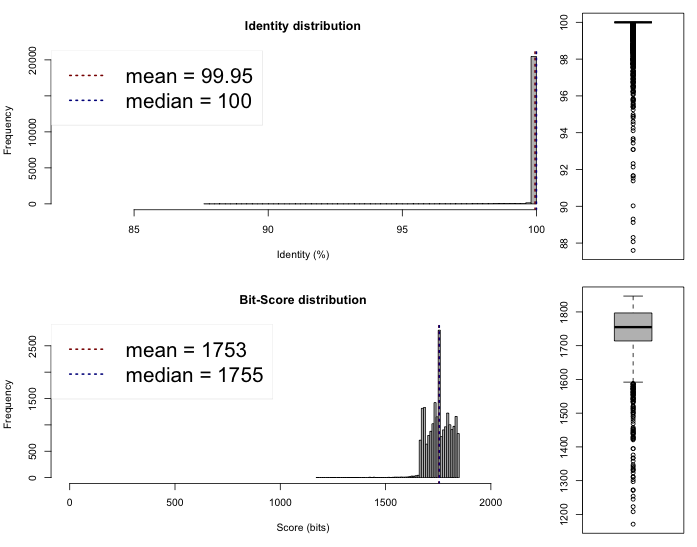
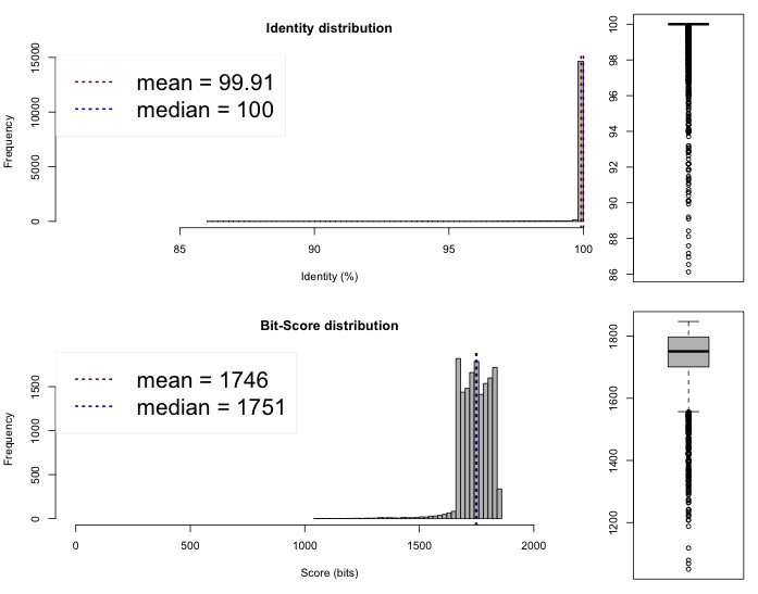
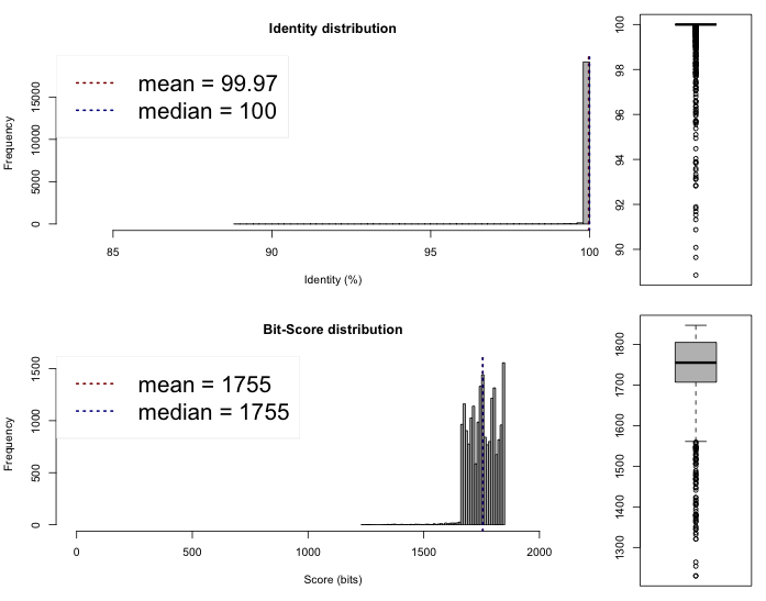
The last thing we can do now is to compare if these draft genomes are different on the sequence level. This can be done rather quickly by comparing the Average Nucleotide Identity, we compared the genomes on the web server of the Kostas Lab. It outputted the following results and plots :
Lib 1 vs 2
One-way ANI 1: 99.93% (SD: 0.58%), from 21582 fragments.
One-way ANI 2: 99.74% (SD: 1.63%), from 23205 fragments.
Two-way ANI: 99.95% (SD: 0.39%), from 21097 fragments.
Lib 1 vs 3
One-way ANI 1: 99.88% (SD: 0.87%), from 16995 fragments.
One-way ANI 2: 99.73% (SD: 1.65%), from 16735 fragments.
Two-way ANI: 99.91% (SD: 0.62%), from 15241 fragments.
Lib 2 vs 3
One-way ANI 1: 99.84% (SD: 1.17%), from 21979 fragments.
One-way ANI 2: 99.95% (SD: 0.57%), from 20025 fragments.
Two-way ANI: 99.97% (SD: 0.32%), from 19473 fragments.
I would say that we assembled three time the same genome here. Which is a good new. Now, these files and especially Lib2 can be sent for annotations to have a look of what is inside and have a quick idea of what we are dealing with !
You can submit your draft genomes for annotation to a number of different annotation servers such as Microscope, Prokka, IMG or RAST. I like RAST for a quick overview because it is the fastest at the moment !
The next blog post will discuss an alternative method to look at these datasets by pooling all the reads related to the gammaproteobacterial contigs and then how to look at the annotations files.
Stay tuned!
And if you have any question, remarks, comment, raging elements to add please leave a comment !
Join the discussion One Comment